CMPUT 503 Exercise 3
Computer Vision
Lens distortion correction
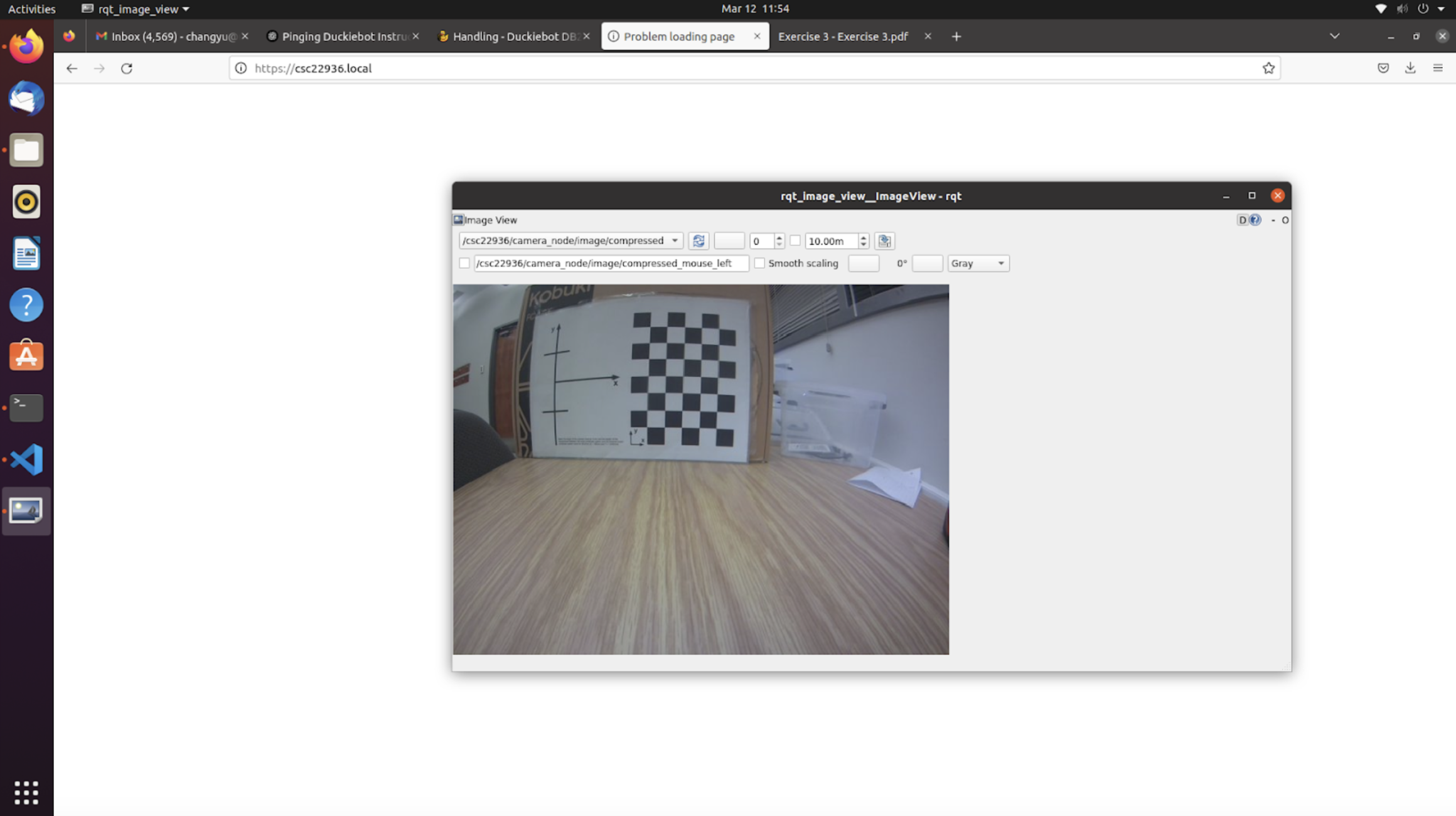

The first image shows the distorted image of the calibration grid caused by lens distortion of the camera. Some curved lines can be spotted for the edges of the objects and the grid lines. The second image shows the undistorted image after undistortion processing using the intrinsic parameters of the camera. The lines of the objects tend to display less of a curvature than the first picture.
Coloured line detection
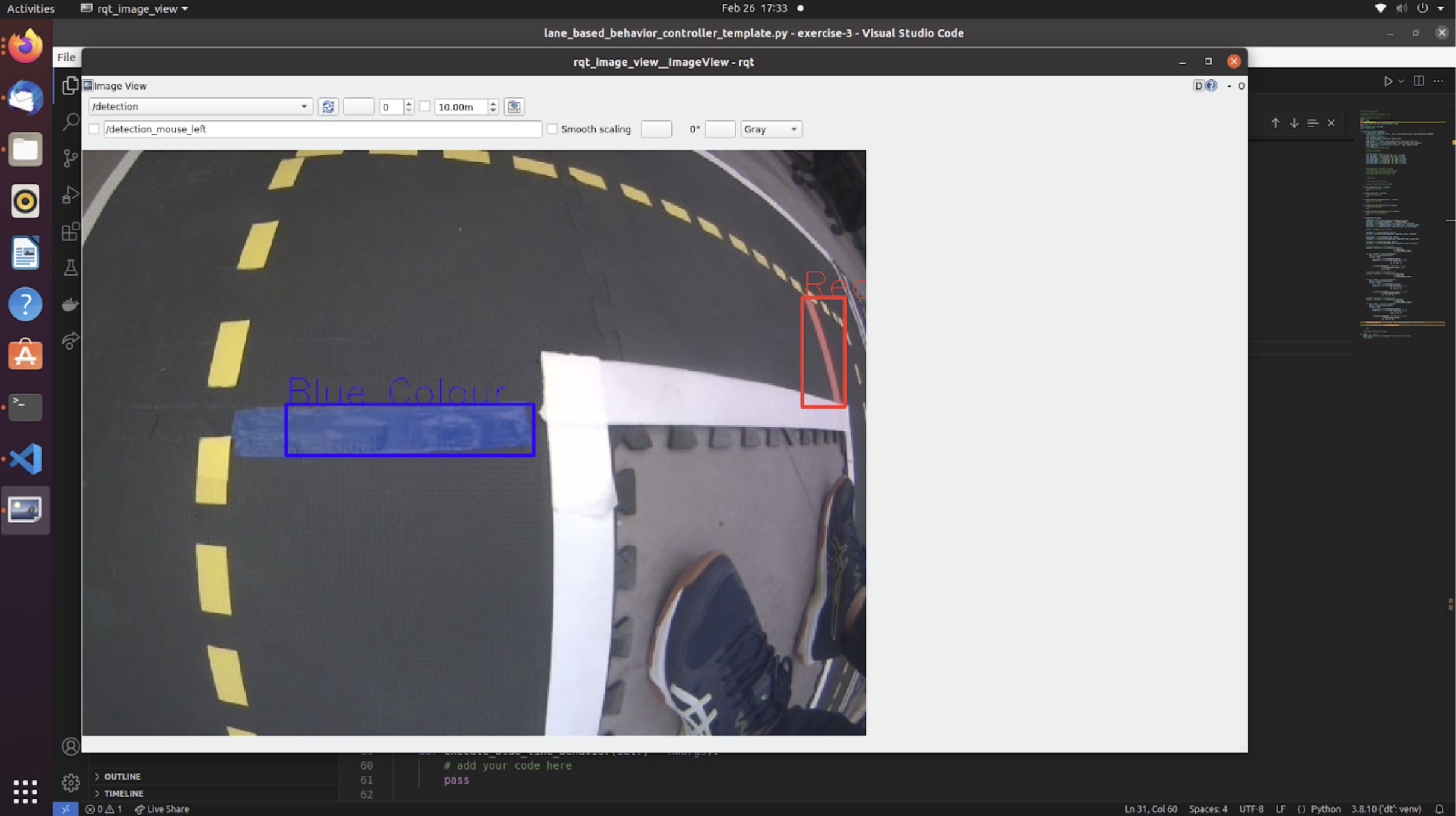
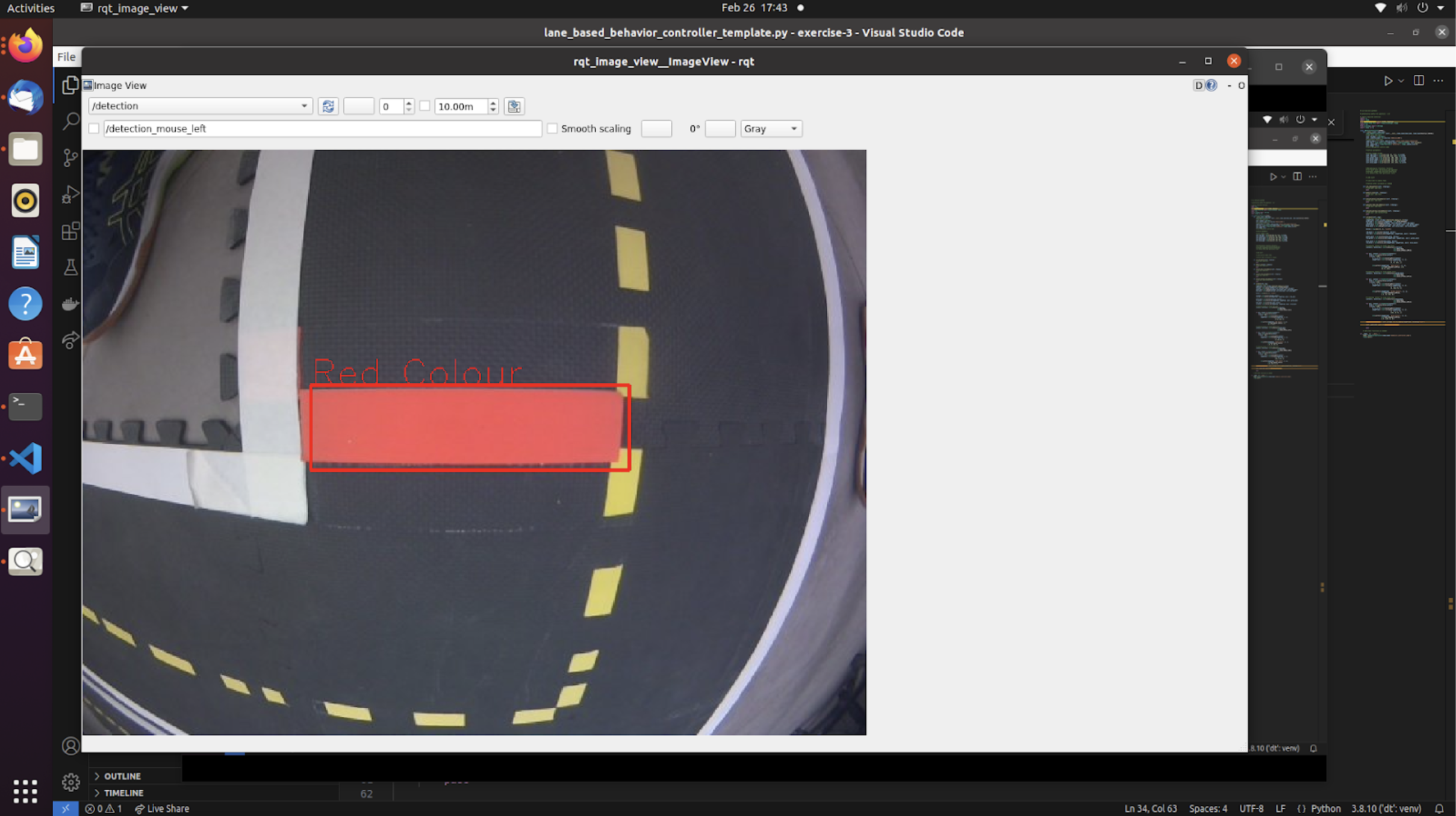
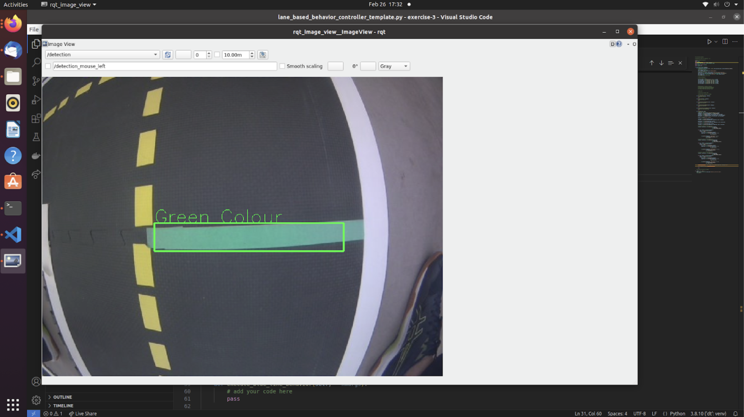
To detect the coloured lines, the camera topic of the Duckiebot is subscribed and HSV colour thresholds for red, blue, and green are determined. The contours of red, blue, and green colour are captured in real-time in the subscribed camera images and are subsequently labeled and published to be a new topic. The above three images are the screenshots of rqt_image_view subscribing to the post-processing topic when the camera is facing at a green, blue, and red line.
How it works
Colour detection works by first defining a lower bound and a upper bound in terms of HSV values. The bounds are turned into a colour mask that is used to find contours with the corresponding colour. The first value in HSV should be selecting the hue of the colour, the second and third value in HSV are for saturation and value, which should be ideally excluding the lower values since those correspond to washed out colours and dark colours. So when tuning HSV parameters for different colours, the hue values should be changed primarily, and the lower bound of the saturation and value can be shifted slightly, while keeping the upper portion of the values relatively the same.
Line detection behaviours
 Link to Video: Red line behaviour
 Link to Video: Green line behaviour
 Link to Video: Blue line behaviour
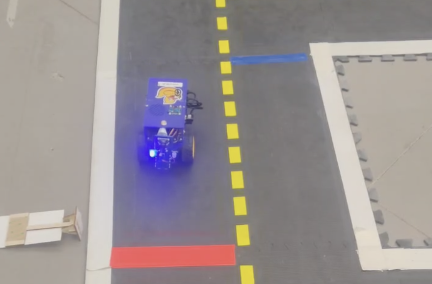
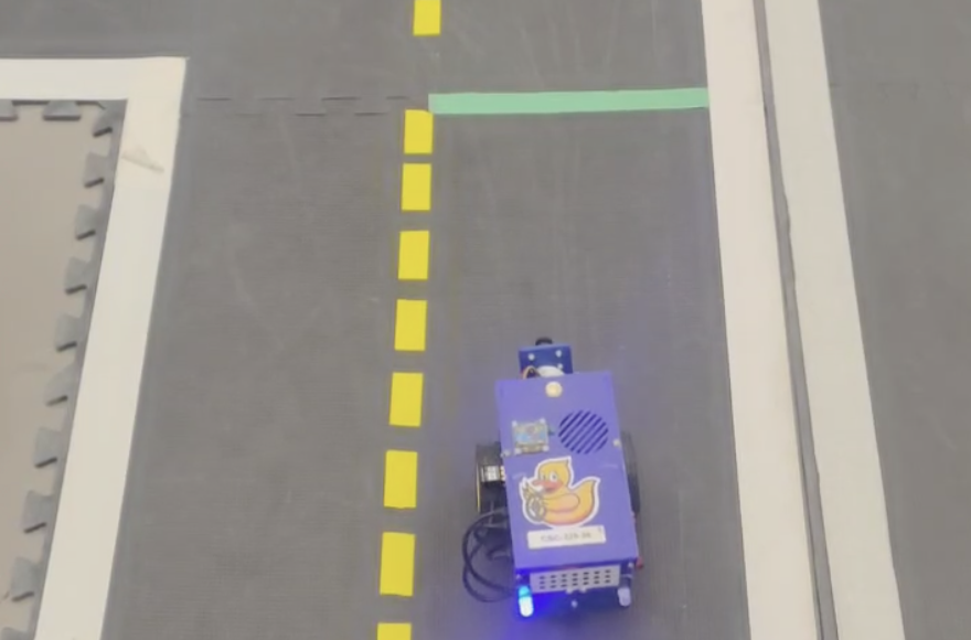
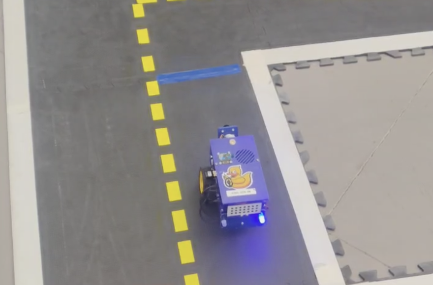
All three videos show Duckiebot being placed 30-50 cm away from a target line. The Duckiebot captures the colour and the contour of the line while moving forward and approaching the line. When the camera does not observe the line anymore (the Duckiebot is very close to the line), it waits for a short interval and initiates a certain behaviour determined by the colour of the previously observed line:
- Red line behaviour: the Duckiebot moves forward for about 50 cm after the pause.
- Green line behaviour: the Duckiebot signals left LEDs and curve towards the left side after the pause.
- Blue line behaviour: the Duckiebot signals right LEDs and curve towards the right side after the pause.
In the video the LED does not change for the green and blue line behaviour. However, in our implemented code, the LED lights do change after the pause, yet they are not reset at each run, thus showing the effect as if the LED lights do not change. When we noticed this, we ran into the RAM issue that prevented us from building on the Duckiebot and re-recording the video, even after multiple attempts and restarts.
Controllers
Videos of Duckiebot driving using P, PD, PID controllers
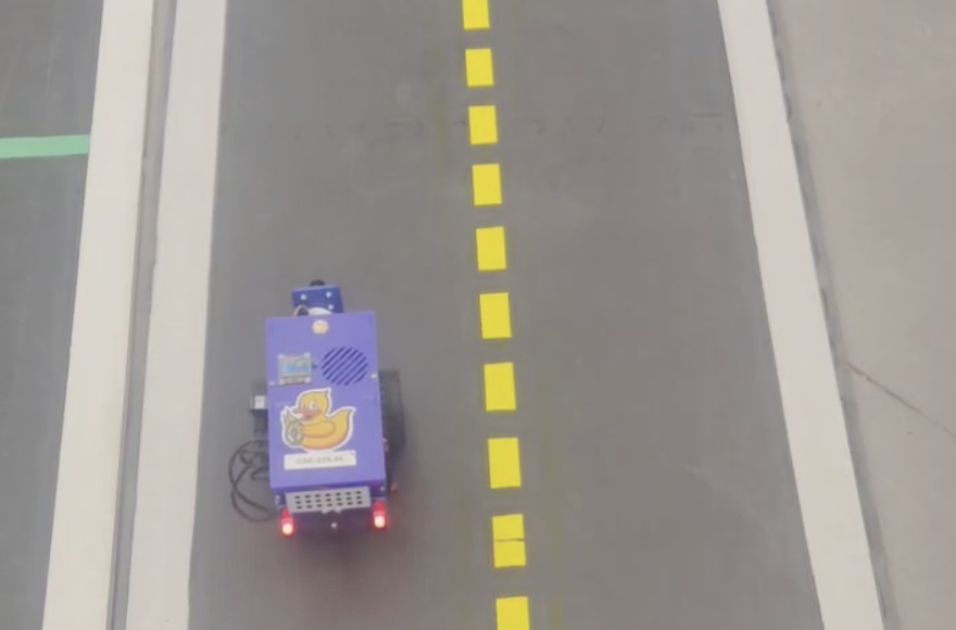

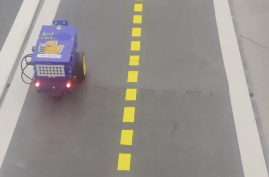
The above videos show the Duckiebot following a straight line for approximately 1.5 m. The Duckiebot detects the white and the yellow line as the boundaries of the lane using its camera, and attempts to stay between the lines by balancing its camera position from the perceived center of the lane. All three controllers take in the proportion of the camera away from the center of the lane as the proportional error and performs changes on wheel controls according to the degree of being off from the center. However, PD and PID also takes in addtional terms to further control the robot driving.
Difference between P, PD, and PID controllers
- P controller takes in the proportional error, tuned by changing the coefficient of the proportional error term.
- PD controller takes in both proportional errors and the rate of change of errors (overshoot), tuned by changing the coefficient of the proportional error term and the derivative error term.
- PID controller takes in proportional errors, accumulation of past errors (steady-state), and the rate of change of errors, tuned by changing the coefficient of the proportional error term, the derivative error term, and the integral error term.
A P controller is the simplest to implement, as it relies only on the current error and a single proportional gain. It provides fast responses and works well for basic tasks like following a straight line. However, it cannot eliminate steady-state error, meaning the system may never reach the exact desired value, and it may struggle with more complex trajectories or disturbances. A PD controller builds on the P controller by adding a derivative term, which reacts to the rate of change of error. This makes the controller more responsive to sudden changes, reducing overshoot and improving stability. However, since it lacks an integral term, it cannot correct for accumulated errors over time, making it less effective for tasks requiring long-term precision. A PID controller combines proportional, integral, and derivative actions to address both transient and steady-state performance. The integral term eliminates steady-state error by accumulating past errors, while the derivative term improves system stability by damping oscillations. This makes PID controllers well-suited for handling both dynamic changes and long-term accuracy. However, they require careful tuning to balance responsiveness, stability, and error correction, making them more complex to configure than P or PD controllers.
Lane Following
Video of lane following
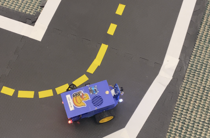
The above video show the Duckiebot performing lane following for a full circle. The P controller is used during the lane following, with the proportional error accounting for the deviation from the center of the lane. When the Duckiebot loses the sight of yellow line in its camera, a default yellow line position is provided as a reference for the duckiebot to calculate a centre of the lane to follow. Depending on the proportional error, the Duckiebot is able to trim the throttle for the wheel on one side, and increase the throttle for the wheel on the other side to adjust its position to remain relatively in the center of the lane.
Write Up
In this project, we (1) converted distorted images to undistorted images, (2) detected lines and colors and obtained the lane dimensions in an image, (3) integrated vision, LED control, and wheel movements, (4) improved and optimized the integrated algorithm, and (5) experimented with P, PD, and PID controllers. We explain what we learned in detail below.
To convert distorted images to undistorted ones, we applied the matrix data of the intrinsic calibration, passed it into the function cv2.getOptimalNewCameraMatrix to get the optimized K and roi, and called the function cv2.undistort to apply those optimized parameters to our image.
To detect colors in the image, we defined the lower and upper HSV range of specified colors, then applied a mask for such ranges over the pixels (in matrix representation) of the image. This returned an image where the pixels with the specified color were masked. We then applied the function cv2.findContours to return the (large enough) contours that were made of those masked pixels. The agent could deduce the lanes from these contours.
In a different method, we tried to detect the edges of the lane. We did that by performing grayscale conversion (required for subsequent actions), Gaussian blurring (for smoothing noise), which was followed by Canny edge detection on the color-masked image. After getting the edges from Canny, we performed Probabilistic Hough Transformation to find important lines. From these lines, we could find lane dimensions by calculating the distance between close and parallel lines. This method didn’t work in lane following as well as we had hoped because of a myriad of “edge” cases.
We integrated vision and wheel movements by allowing the agent to publish vertical wheel velocities to the wheel topics, reacting to what it saw from the camera subscriber. We integrated LED control into the pipeline by creating a publisher that published to the topic subscribed to by the four LEDs of the bot.
The whole process was optimized by tuning hyperparameters such as KP and KD for P, PD, and PID controllers, as well as the wheels’ speed. We cut irrelevant parts of the image away. We introduced a clipping technique that prevented the agent from turning the wheels too fast too suddenly (which could have happened due to the camera’s latency and inaccuracies). We introduced a hyperparameter that allowed us to translate how much the controller’s signaled error corresponded to the wheel’s new speed. In our experiment, the default camera frequency and control update rate worked perfectly. If the camera frequency had been much faster, it could have throttled the wheel movement and vision processing program; if it had been much slower, the wheel controller would have required tuning accordingly (for example, if the frame rate was slow, we would have had to define approximate movements between frames).
Now we analyzed the three types of controllers. P was the simplest to implement and tune. It returned the most recent error—straightforwardly. PD incorporated the change in the recent errors. This “D” was calculated by taking the difference between the previous error and the current error (multiplied by the timestep, of course). This helped with predicting the next change based on this rate of change. By considering the rate of change, PD had the advantage that it could eliminate overshooting errors. PID incorporated the total error over time and thus helped reduce steady-state errors (the error that was measured when the system stabilized). The “I” was calculated by summing up all the errors (multiplied by the timestep) that built up over time. This method helped because it generalized the system’s overall tendency into its controller. However, it was more complicated to tune, and it could overfit to any accidental steady-state errors that occurred in the past.
In our experiment, the derivative and the integration didn’t help. The reason was that our robot received plenty of real-time feedback and could react very quickly already, so overshooting errors and built-up errors were not problematic.
So we used P predominantly in our experiment. With P, tuning was simple because the magnitude of the error was linearly proportional to what the controller should do. So having a multiplier and clipping was enough. The error was calculated using a formula on the x and y coordinates of the nearest white and yellow contours. The x-coordinates signified the lateral error of the bot. The y-coordinates signified the rotational error of the bot. This setup worked well for both straight-line and curved-lane following without needing to introduce D and I into the controller.
References
Collboration
- The report is a joint effort by Alex Liu and Minh Pham on the completed deliverables of the lab, including the aformentioned screenshots and video, as well as the github repository.
- Questions regarding the lab were answered by TAs of the course.
AI Usages
- ChatGPT and DeepSeek was used to reword some sentences in this report and to assist in coding.